Build the data entry form for a time tracking app using Google Sheet (part 1 of 3)

Welcome to part 1 of this tutorial. We’ll build the data entry form for a time tracking app using Google Sheets. For an overview of the project, please see the Time Tracker guide.

step 1. create the data entry form

Let’s start by building a data entry form in a new Google Sheet for a single day.

• Create a new Google Sheet (from Google Drive or by typing sheets.new in your browser’s URL bar).
• Rename the sheet (by double-clicking the tab at the bottom) to “Tracker”.
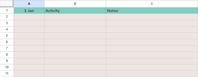
• Create a header row with today’s date, “Activity”, and “Notes”.
• Using a color of your choice, color the next 10-15 rows to indicate they are data entry cells.

Here’s what mine looks like:

step 2. add formatting and data validation

Column A will be where we enter the time at which we begin our day and any time we switch tasks. Let’s format that range and set data validation to ensure we enter a valid time.

• Select your data entry range for column A ( A2:A11 in my sheet).
• Select Format > Number > Custom date and time from the menu bar to input a custom format. Set the format as Hour (1) : Minute (01). (You can adjust this to a format you prefer later, but follow along for now.) Here’s what it should look like:

Column B with header “Activity” will be where we enter the name of the task we’re working on. We’ll want to make sure that we enter the same task name each time. Let’s create a dropdown validation from a range that we can populate with task names.

• First, add a new sheet to store the task names (click the plus icon at the bottom left of the application window). Name the sheet “Tasks”.
• In the first row, add header names “Name” and “Category”.
• Populate column A with a list of tasks you will be tracking.
• Categorize each task in column B. I’ll use the categories “Work”, “Personal Projects”, and “Areas” based on the Getting Things Done or PARA productivity systems. You can use any categories that resonate with you, but I recommend no more than 5-7 categories to be meaningful. We’ll use these categories to aggregate hours tracked for a “rolled-up” view of what we are spending time on.
• Importantly, include a task named “BREAK” (no category needed). We’ll use this task when we want to, well, take a break.

Here’s an example of the Tasks sheet:

I like to delete any columns I’m not using from a Google Sheet, feel free to delete columns C and onward if you’d like.

Now, let’s return to the Tracker sheet and set up the dropdown data validation.

• In the Tracker sheet, select the data entry range for the Activity column (B2:B11 in my sheet).
• Select Format > Data > Data Validation to open the Data validation rules sidebar.
• Select “Dropdown (from a range)” as the Criteria.
• Set the range to =Tasks!$A$2:$A.
• Under Advanced Options, set Display style to Arrow (or use your preferred style).

step 3. calculate hours per entry

Let’s input some dummy data to help us as we build out the formulas that will aggregate time for the day.

• In cell A2, input your start time for the day.

• In cell A3, select a task.
• Add notes describing what you were working on for each task.
• Repeat these steps to create a handful of tasks.

Next, we’ll add two helper columns to calculate the duration of each task.

• In column D, add the header “Date” and format the range below using your preferred date format.
• In column E, add the header “Hours” and format as a number with two decimal places.
• Column D will simply be a helper column that repeats the date from cell A1. Add the following formula to cell D2:

=ARRAYFORMULA(IF(ISBLANK(A2:A11),,A1))

Column E will calculate the duration between the start time and the next start time, giving us the duration we worked on the previous task. We want to use an array formula (for reasons we’ll see shortly), but let’s build up to our array formula in steps.

• First, input the following formula into cell E2. This formula calculates the duration between the two start times in fractions of a day. We multiply by 24 to get hours.

=IF(ISBLANK(A3),,(A3-A2)*24)

• Next, let’s adapt the formula to work with arrays rather than copy the formula through the column. The only change we need to make is to wrap the current formula in ARRAYFORMULA() and change the individual cell references to array references. Here is the final formula for cell E2.

=ARRAYFORMULA(IF(ISBLANK(A3:A11),,(A3:A11-A2:A10)*24))

You should now see the date from cell A1 and the total hours spent on each task in each row. Here’s what mine looks like:

The reason we use array formulas will become clear in the next step, where we’ll duplicate the day’s data entry form to complete a full week. If we had used regular formulas, we would need to manually change the range references for each day. With array formulas, we don’t need to do anything!

step 4. duplicate daily data entry form for the week

To complete our data entry form, let’s duplicate the daily data entry form for each day of the week.

• First, group the rows for the day. Select all rows 2:11 and select View > Group from the menu bar (or right-click the numbered rows along the left-hand side and select group or use the hotkey Alt + Shift + ->).
• Select all rows 1:11 and press Ctrl + C to copy.
• Select cell A12 and paste by pressing Ctrl + V.
• Update cell A12 with the formula =A1+1. The cell should now show the date after the date shown in cell A1.
• Select all rows 12:22, copy and paste into cell A23.
• Continue copying and pasting until you have created the data entry form for a full week (seven days).

up next

Congratulations on setting up the Time Tracker! In part 1 of this tutorial, you set up a basic data entry form as a table in Google Sheets, applied formatting and data validation, and practiced with array formulas.

You can access a copy of the Time Tracker based on this tutorial here. Please click the USE TEMPLATE button to make a copy into your own Google Drive.

In the Time Tracker - part 2, we’ll use Google Apps Script to automate the process of logging the data at the end of each week and clearing out the data entry form for the next week.